File:2014rubleDollar3param.png

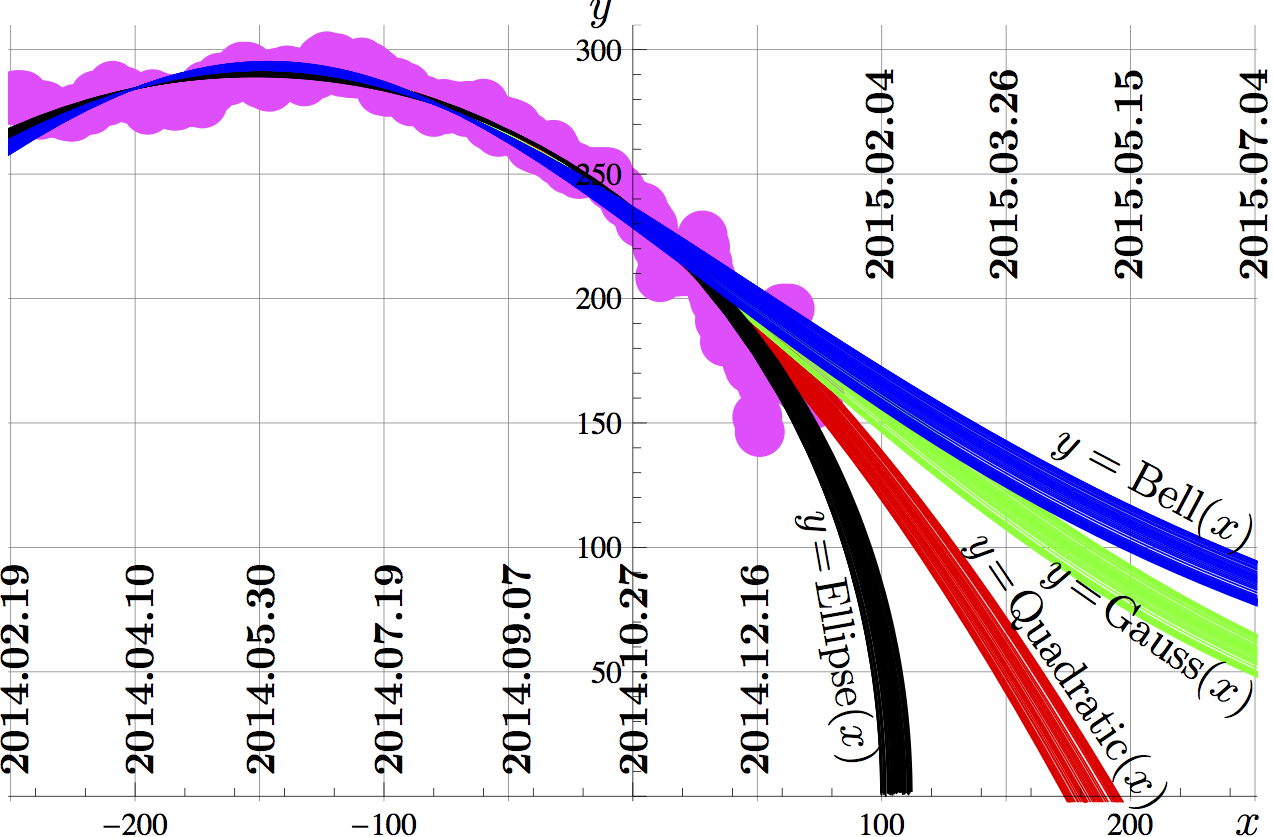
Price of 100 Russian roubles, evaluated in the USA cents, versus time.

This figure appears as fig.2 in publication ^[1].

Data since 2014.02.20 to 2015.01.09 (the date of submission) are considered.

Time \(x\) is measured in days since the beginning of the project, 2014.10.27.

Pink dots represent the experimental data by https://www.mataf.net/en/currency/converter-USD-RUB

The thick smooth lines are formed by the four sets of approximations. Each set is formed with specific 3-parametric function \(f\), and values of parameters are chosen to minimize the mean square deviation

\(\displaystyle Q=\sqrt{ \sum_{n=1}^m \big(F_n-f(X_n)\big)^2 }\)

for \(M-50\le m\le M\), where \(M\) is total number of experimental dots available for the day of plotting. For each \(m\), the single curve is drawn, emulating situation when the data with number larger \(m\) are not yet available. With growth of \(m\), the evolution of the approximation with time can be traced. The thickness of the resulting line qualifies the instability of the approximation.

In the way mentioned above, the following four functions \(f\) are considered and plotted:

\(f(x)=\mathrm{Bell}(x) = a\ /\cosh(b(x+c))\)

\(f(x)=\mathrm{Gauss}(x) = a \exp(b x+c x^2))\)

\(f(x)=\mathrm{Quadratic}(x) = a + b x +c x^2\)

\(f(x)=\mathrm{Ellipse}(x)=a \sqrt{(b-x)(c+x)}\)

For these functions, the mean square deviations is of order of 10.

The input data are stored as array of pairs \(X_n\), \(F_n\) ; the input file is loaded at https://mizugadro.mydns.jp/t/index.php/File:Roublellip.png#Data

Mathematica generator of lines

g0 = Import["~/Q/RUBLE/BUL/TRY01/ddat.txt", "Table"];
T0[i_] := Extract[Extract[g0, i], 1];
G0[i_] := Extract[Extract[g0, i], 2]; M0 = Length[g0]

lp = ListPlot[g0, PlotRange -> All, PlotStyle -> {RGBColor[1, 0, 1], PointSize[.04]}]

For[i = M0 - 52, i < M0, i++; Print[i]; 
 g = Table[{T0[j], G0[j]}, {j, 1, i}]; M = Length[g];
 T[i_] := Extract[Extract[g, i], 1];
 G[i_] := Extract[Extract[g, i], 2];
 F[x_] = a + b x + c x^2; sub = FindFit[g, F[x], {a, b, c}, x];
 Print[{f[x_] = ReplaceAll[F[x], sub], ReplaceAll[a, sub], 
   ReplaceAll[b, sub], ReplaceAll[c, sub],
   Sum[Abs[f[T[i]] - G[i]], {i, 1, M}]/M, 
   Sqrt[Sum[(f[T[i]] - G[i])^2, {i, 1, M}]/M],
   plo31[i] = 
    Plot[f[x], {x, -260, 201}, PlotStyle -> {RGBColor[1, 0, 0]}, 
     PlotRange -> All]; Show[lp, plo31[i]]}]
 ]

For[i = M0 - 52, i < M0, i++; Print[i]; 
 g = Table[{T0[j], G0[j]}, {j, 1, i}]; M = Length[g];
 T[i_] := Extract[Extract[g, i], 1];
 G[i_] := Extract[Extract[g, i], 2];
 F[x_] = 300 a Exp[-.1 b x - .01 c x^2]; 
 sub = FindFit[g, F[x], {a, b, c}, x];
 Print[{f[x_] = ReplaceAll[F[x], sub], ReplaceAll[a, sub], 
   ReplaceAll[b, sub], ReplaceAll[c, sub],
   Sum[Abs[f[T[i]] - G[i]], {i, 1, M}]/M, 
   Sqrt[Sum[(f[T[i]] - G[i])^2, {i, 1, M}]/M],
   plo32[i] = 
    Plot[f[x], {x, -261, 261}, PlotStyle -> {RGBColor[0, 1, 0]}, 
     PlotRange -> All]; Show[lp, plo32[i]]}]
 ]

Show[lp, Table[plo31[n], {n, M0 - 51, M0}], 
 Table[plo32[n], {n, M0 - 51, M0}], 
 PlotRange -> {{-261, 201}, {-2, 310}}, AspectRatio -> Automatic, 
 GridLines -> Automatic]

For[i = M0 - 52, i < M0, i++; Print[i]; 
 g = Table[{T0[j], G0[j]}, {j, 1, i}]; M = Length[g];
 T[i_] := Extract[Extract[g, i], 1];
 G[i_] := Extract[Extract[g, i], 2];
 F[x_] = 300 a Sqrt[(100 + b - x) (400 + c + x)]; 
 sub = FindFit[g, F[x], {a, b, c}, x];
 Print[{f[x_] = ReplaceAll[F[x], sub], ReplaceAll[a, sub], 
   ReplaceAll[b, sub], ReplaceAll[c, sub],
   Sum[Abs[f[T[i]] - G[i]], {i, 1, M}]/M, 
   Sqrt[Sum[(f[T[i]] - G[i])^2, {i, 1, M}]/M],
   plo33[i] = 
    Plot[f[x], {x, -261, 261}, PlotRange -> All, 
     PlotStyle -> RGBColor[0, 0, 0]]; Show[lp, plo33[i]]}]
 ]

Show[lp, Table[plo31[n], {n, M0 - 51, M0}], 
 Table[plo32[n], {n, M0 - 51, M0}], Table[plo33[n], {n, M0 - 51, M0}],
  PlotRange -> {{-261, 201}, {-2, 310}}, AspectRatio -> Automatic, 
 GridLines -> Automatic]

For[i = M0 - 52, i < M0, i++; Print[i]; 
 g = Table[{T0[j], G0[j]}, {j, 1, i}]; M = Length[g];
 T[i_] := Extract[Extract[g, i], 1];
 G[i_] := Extract[Extract[g, i], 2];
 F[x_] = 300 a /Cosh[.01 b (100 + c + x)]; 
 sub = FindFit[g, F[x], {a, b, c}, x];
 Print[{f[x_] = ReplaceAll[F[x], sub], ReplaceAll[a, sub], 
   ReplaceAll[b, sub], ReplaceAll[c, sub],
   Sum[Abs[f[T[i]] - G[i]], {i, 1, M}]/M, 
   Sqrt[Sum[(f[T[i]] - G[i])^2, {i, 1, M}]/M],
   plo34[i] = Plot[f[x], {x, -261, 261}, PlotRange -> All, 
     PlotStyle -> RGBColor[0, 0, 1]]; Show[lp, plo34[i]]}]
 ]

p3 = Show[lp, Table[plo31[n], {n, M0 - 51, M0}], 
  Table[plo32[n], {n, M0 - 51, M0}], 
  Table[plo33[n], {n, M0 - 51, M0}], 
  Table[plo34[n], {n, M0 - 51, M0}], 
  PlotRange -> {{-251, 251}, {-2, 310}}, AspectRatio -> Automatic, 
  GridLines -> {{-250, -200, -150, -100, -50, 50, 100, 150, 200, 
     250}, {50, 100, 150, 200, 250, 300}}]

Export["p34.pdf", p3]

C++ generator of dates

Latex generator of labels

\documentclass[12pt]{article} 
\usepackage{geometry}
\paperwidth 368pt
\paperheight 242pt
\topmargin -66pt
\oddsidemargin -70pt
\usepackage{hyperref}
\usepackage{graphicx}
\usepackage{rotating}
\newcommand \sx {\scalebox}
\newcommand \rot {\begin{rotate}}
\newcommand \ero {\end{rotate}}
\thispagestyle{empty}
\parindent 0pt
\begin{document} 
\begin{picture}(400,200)
\put(0,0){\includegraphics{p34}}
\put(6,19){\sx{1.}{\rot{90}{\bf 2014.02.19}\ero}}
\put(42,19){\sx{1.}{\rot{90}{\bf 2014.04.10}\ero}}
\put(77,19){\sx{1.}{\rot{90}{\bf 2014.05.30}\ero}}
\put(114,19){\sx{1.}{\rot{90}{\bf 2014.07.19}\ero}} %
\put(151,19){\sx{1.}{\rot{90}{\bf 2014.09.07}\ero}} %
\put(185,19){\sx{1.}{\rot{90}{\bf 2014.10.27}\ero}} %
%\put(220,19){\sx{1.}{\rot{90}{\bf 2014.12.16}\ero}} %
%\put(256,19){\sx{1.}{\rot{90}{\bf 2015.02.23}\ero}}
%\put(292,19){\sx{1.}{\rot{90}{\bf 2015.04.13}\ero}}
%\put(328,19){\sx{1.}{\rot{90}{\bf 2015.05.15}\ero}}
%\put(364,19){\sx{1.}{\rot{90}{\bf 2015.07.04}\ero}}
\put(168,238){\sx{1.1}{$y$}}
%\put(324,163){\sx{1.1}{\rot{-4}$f_{23}(x)$\ero}}
%\put(324,150){\sx{1.1}{\rot{-6}$f_{22}(x)$\ero}}
\put(302,114){\sx{1.1}{\rot{-28}$y=\mathrm{Bell}(x)$\ero}}
\put(299,77){\sx{1.1}{\rot{-35}$y\!=\!\mathrm{Gauss}(x)$\ero}}
\put(277,86){\sx{1.1}{\rot{-56}$y\!=\!\mathrm{Quadratic}(x)$\ero}}
\put(230,95){\sx{1.1}{\rot{-80}$y\!=\!\mathrm{Ellipse}(x)$\ero}}
%\put(190,105){\sx{1.2}{experimental}}
%\put(204,92){\sx{1.2}{data}}
\put(355,2){\sx{1.1}{$x$}}
\end{picture}
\end{document}

References

Keywords

«Fraud», «Inflation», «Insider trading», «Moscovia», «Pump and down», «Ruble», «TrumptyDumpty»,

«Инфляция», «Коррупция», «Московия», «Рубль»,

References

- ↑ https://www.m-hikari.com/ams/ams-2015/ams-17-20-2015/kouznetsovAMS17-20-2015.pdf Dmitrii Kouznetsov. Currency Band and the Approximations: Fitting of Rouble with 3-Parametric Functions. Applied Mathematical Sciences, Vol. 9, 2015, no. 17, 831 - 838 HIKARI Ltd, www.m-hikari.com http://dx.doi.org/10.12988/ams.2015.4121056